Item similarity derived from receipts: an embedding approach
This blog describes the basic principle of using the embedding method to derive the item similarity from receipts. The implementation is done with python + pandas + scipy.
Raw data
The schema of the sample data:
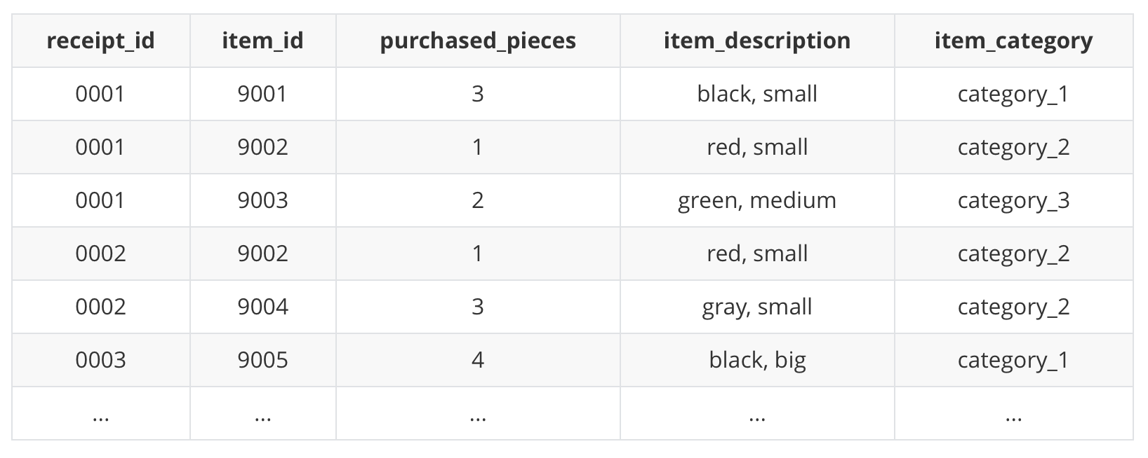
Typically, a receipt is associated with a receipt_id, where one or more item_id will be listed on the receipt together with purchased_pieces, item_description and item_category.
Note that only
receipt_id,item_idandpurchased_piecesare needed to derive the item similarity.item_descriptionanditem_categoryare used for the visual representation.
import itertools
import pandas as pd
import numpy as np

raw_receipt_df = pd.read_csv("sample_data.csv", sep='|')
Data cleaning
Despite the quality of your raw data, we need to remove the receipts that contains only 1 item because those receipts are not useful to build the point-wise mutual information (PMI).
raw_receipt_df.columns = raw_receipt_df.columns.str.lower()

receipt_df = (
    raw_receipt_df.groupby(["receipt_id", "item_id"])["purchased_pieces"]
    .sum()
    .reset_index()
)

def filter_receipt(df, thredhold=1):
    counts = df.groupby(["receipt_id"])["item_id"].count()
    df = df.set_index("receipt_id")
    df = df[counts > thredhold]
    df = df.reset_index()
    return df

receipt_df = filter_receipt(receipt_df)
Construction of the point-wise mutual information (PMI)
The PMI is defined as: \(\text{PMI}(x; y) = log_2 \frac{p(x y)}{p(x)p(y)}\)
The normalized PMI (nPMI) is defined as: \(\text{nPMI} = \frac{\text{PMI}(x; y)}{-log_2p(X=x)}\)
def get_cocurrence_counts(df, i1, i2):
    tempdf = df[df.item_id.isin([i1, i2])]
    cocurrence = len(tempdf) - tempdf.receipt_id.nunique()
    return cocurrence

def get_pmi(df):
    item_counts = df.item_id.value_counts()
    n_total = len(df)

    n_i1i2 = []
    for i1, i2 in itertools.combinations(item_counts.index, 2):
        n_i1i2.append((i1, i2, get_cocurrence_counts(df, i1, i2)))

    pmi_df = pd.DataFrame(n_i1i2, columns=["i1", "i2", "n_i1i2"])

    pmi_df["n_i1"] = pmi_df.i1.map(item_counts)
    pmi_df["n_i2"] = pmi_df.i2.map(item_counts)
    pmi_df["PMI"] = np.log(pmi_df.n_i1i2 / (pmi_df.n_i1 * pmi_df.n_i2) * n_total)

    log_p_i1_p_i2 = np.log(pmi_df.n_i1 * pmi_df.n_i2 / (n_total * n_total))
    log_p_i1i2 = np.log(pmi_df.n_i1i2 / n_total)
    pmi_df["nPMI"] = log_p_i1_p_i2 / log_p_i1i2 - 1

    pmi_df = pmi_df[["i1", "i2", "PMI", "nPMI"]]
    return pmi_df

pmi_df = get_pmi(receipt_df)
Filter the ones with nPMI > 0:
pmi_df = pmi_df[pmi_df.nPMI > 0]
PMI embedding with singular value decomposition (SVD)
Construct the PMI sparse matrix.
from scipy.sparse import csc_matrix, csr_matrix
import scipy.sparse.linalg, scipy.sparse

item2index = dict((item, i) for i, item in enumerate(set(pmi_df.i1) | set(pmi_df.i2)))
index2item = dict(enumerate(set(pmi_df.i1) | set(pmi_df.i2)))

pmi_df["index1"] = pmi_df.i1.map(item2index)
pmi_df["index2"] = pmi_df.i2.map(item2index)

data = pmi_df.PMI.append(pmi_df.PMI, ignore_index=True)
row_ind = pmi_df.index1.append(pmi_df.index2, ignore_index=True)
col_ind = pmi_df.index2.append(pmi_df.index1, ignore_index=True)
pmi_sparse = scipy.sparse.csr.csr_matrix((data, (row_ind, col_ind)))
Perform SVD on PMI matrix. However this matrix is very long and sparse. In many scenarios, it is beneficial to convert this long and sparse matrix into a short and dense representation.
The truncated singular value decomposition is applied to the PMI sparse representation.
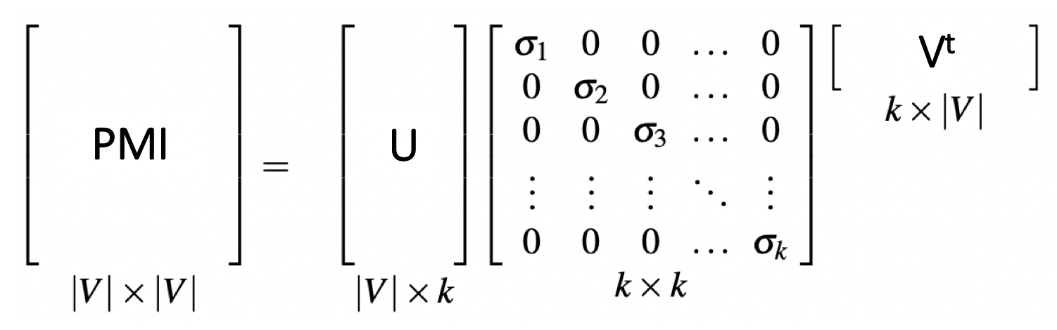
U, S, Vt = scipy.sparse.linalg.svds(pmi_sparse, k=10, which='LM')
Depends on your application, generally the top k (k=10, which='LM') dimensions are used. Each row in U is the corresponding embedding for each item, namely each item is embedded by a k=10 dimensional vector.
Cosine similarity calculation
The cosine similarity is used to score the item similarity.
from sklearn.metrics.pairwise import cosine_similarity
similarity_matrix = cosine_similarity(U)
Visualization of the embedding with t-SNE
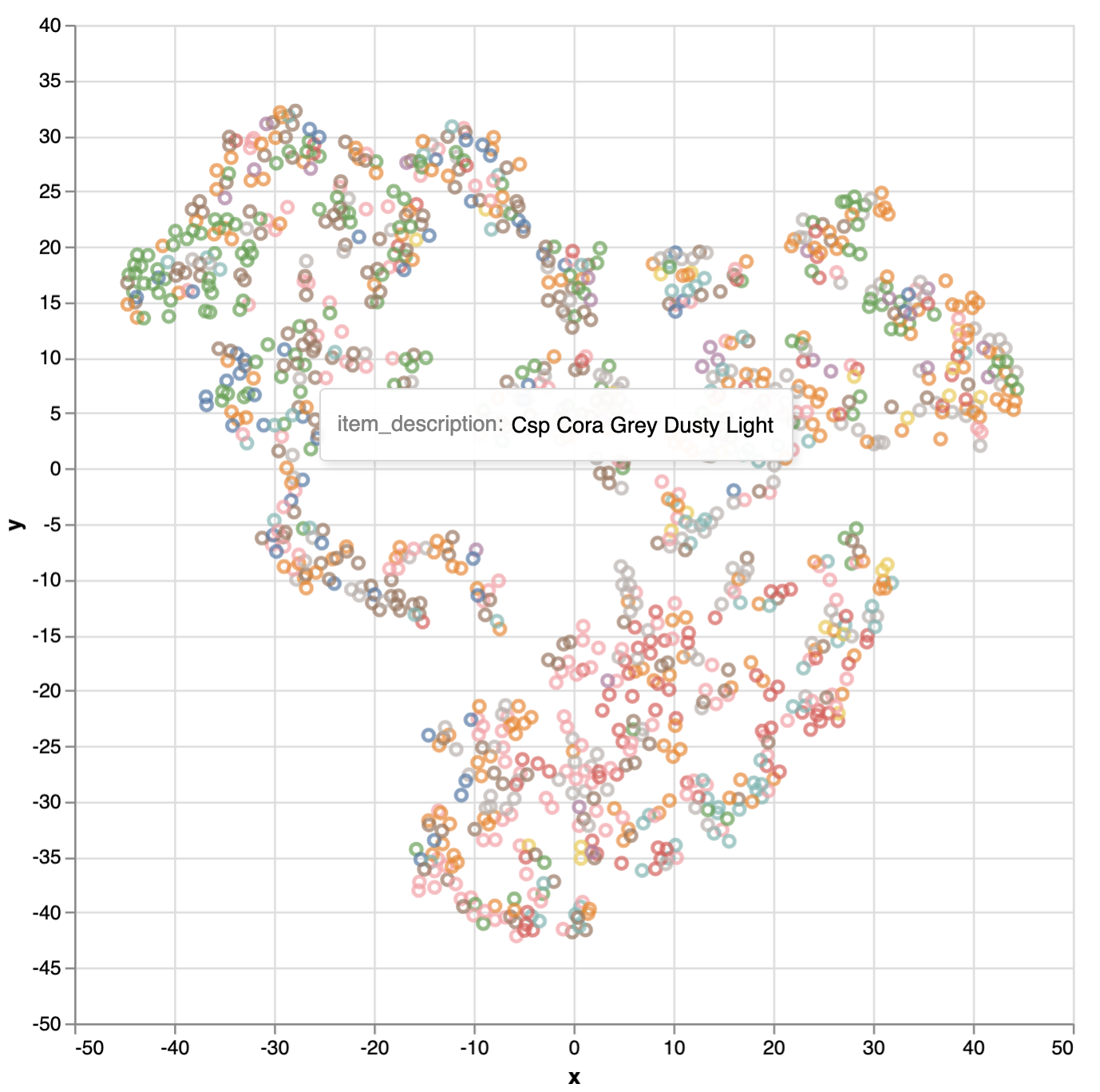
Dimension reduction with t-SNE. The t-distributed Stochastic Neighbor Embedding (t-SNE) is used to visualize the high-dimensional data that will be embedded into 2 or 3 dimensions.
The purpose of t-SNE visualization is to have a human intuitive validation on the embedding, which should NOT be taken as any quantitative similarity measure.
from sklearn.manifold import TSNE

tsne = TSNE(n_components=2, random_state=42)
U_2d = tsne.fit_transform(U)
Interactive visualization. By using Vega, we can interactively visualize the embedding. Below the item embeddings are colored by the item category. It clearly shows the clustering of item category as expected.
vis_df = pd.DataFrame(U_2d, columns=["x", "y"])
vis_df["item_id"] = vis_df.index.map(index2item)
item_df = raw_receipt_df[
    ["item_id", "item_description", "item_category"]
].drop_duplicates()
vis_df = vis_df.merge(item_df, how="left", on="item_id")
from vega import VegaLite

VegaLite(
    {
        "mark": "point",
        "width": 400,
        "height": 400,
        "encoding": {
            "y": {"type": "quantitative", "field": "y"},
            "x": {"type": "quantitative", "field": "x"},
            "color": {"type": "nominal", "field": "item_category"},
            "tooltip": [{"type": "nominal", "field": "item_description"}],
        },
    },
    vis_df,
)
Summary
A simple pipeline, utilizing the embedding of the item-item PMI, is introduced to derive the item similarity based on the sale receipts data. This item similarity approach goes beyond the visual similarity between the items, where it potentially takes into account price, etc.