Visual similarity from a controlled embedding approach
Note that the following discussion will be focus on the
visual similarity, meaning that all the information you can extract from the image of the object. For example, the price of the object is not in the scope of discussion.
Introduction
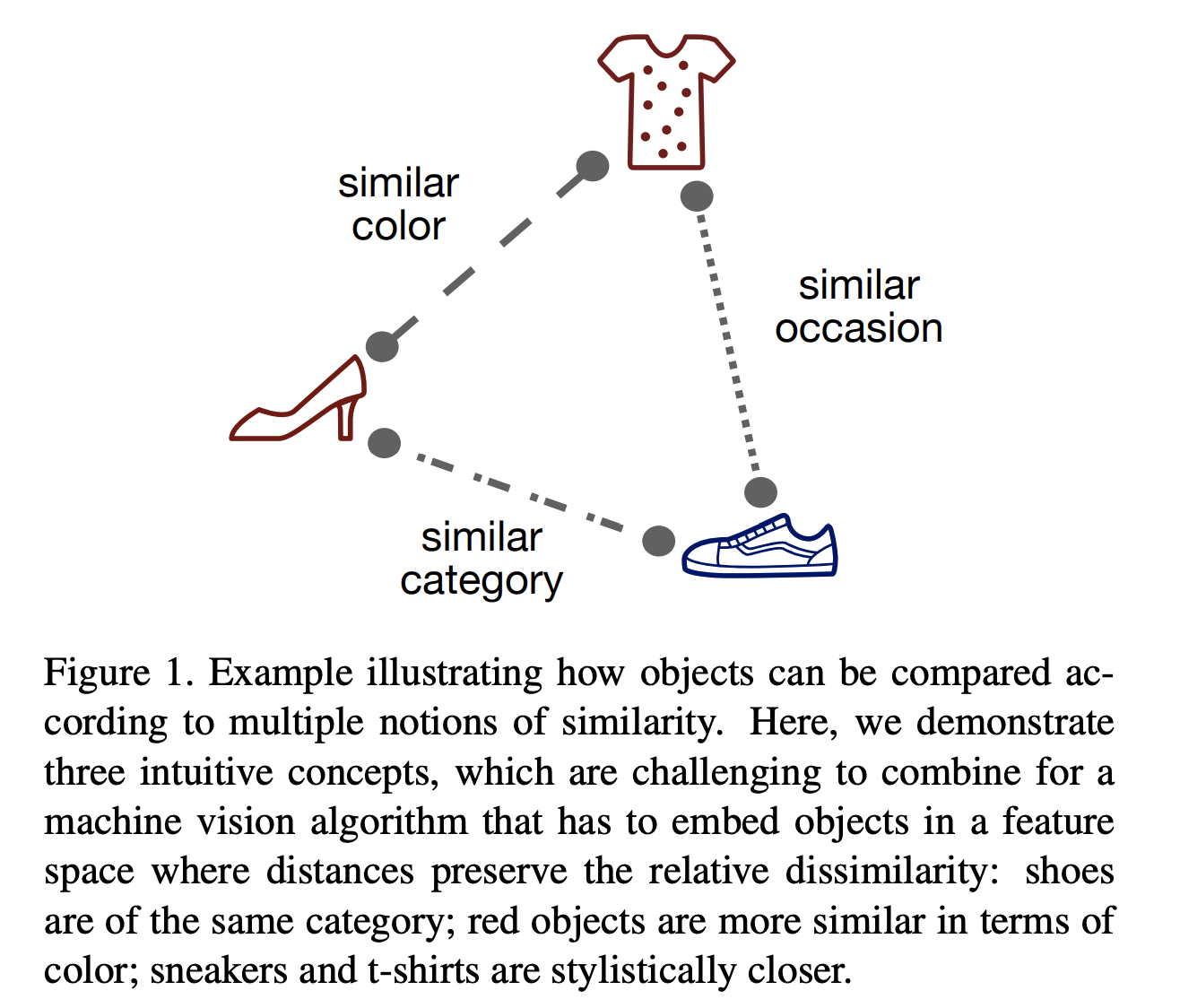
Visual similarity is an important building block in many machine learning systems, such as recommendation system, image retrieval system. However, depending on the applications, the semantic definition of visual similarity varies a lot. Below is an illustration of different notions of visual similarity from Veit 2017. Therefore it is important to specify the semantic definition of visual similarity when discussing the topics around visual similarity.
Note that I will use the term
conditional visual similarityto refer to the semantic definition of visual similarity in the following discussion.
Once the conditional visual similarity is defined, we are in the position to measure the similarity between objects. To measure the visual similarity between objects, the images of the objects are typically embedded in a feature-vector space, where the distances, such as cosine distance, between the vectors are derived as the relative dissimilarity.
The image embedding can be derived from both supervised and un-supervised fashion. In the supervised approach, either the pairwise Chopra 2005 or triplet Wang 2014 loss functions are chosen to supervise the learning, which requires a large amount of labelled data set or a well-designed way to generate training data. On the other hand, the un-supervised approach typically involves certain pre-trained neural network architecture, where the last layer is replaced by the embedding layer, to carry out one-shot learning.
In this article, I will illustrate both a supervised and an un-supervised approach to derive the image embedding, and calculate the cosine similarity using a publicly available fashion data sets Kaggle: Fashion Product Images Dataset. The implementation will be done with pytorch and can be found on my github.
What’s image and similarity?
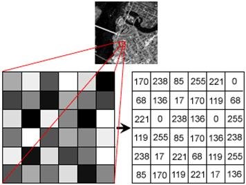
Image. An image is basically an array of size [n_channels, width, length], where an element of the array is an integer ranging from 0 to 255, as shown above.
Similarity. Roughly speaking, similarity is a measure of the difference between
two matrices. However depending on the condition of the similarity, a
transformation is needed to bring the image from one state to anther state as shown
above. This transformer is basically the implementation of the condition.
Because the condition can be defined differently in difference applications, we
will end up different transformers.
Similarity from the controlled embedding: Implicitly vs Explicitly
With a well-defined condition, the problem can be tackled either from an un-supervised or a supervised fashion. While the un-supervised approach implicitly encodes the condition, the supervised one explicitly expresses the condition.
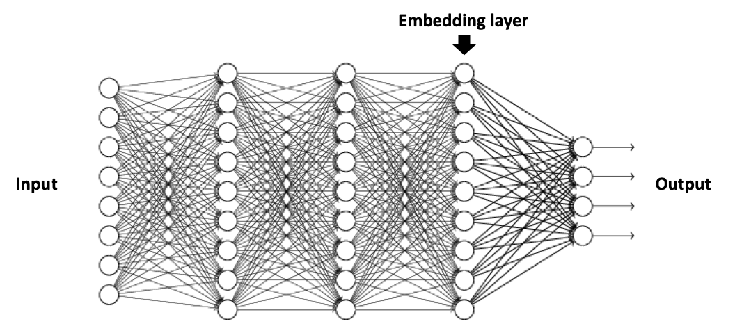
Implicitly controlled embedding. This method takes a pre-trained neural
network and passes an image into the network to get the embedding vectors as shown
below. Note that no fine-training is necessarily required. Depending on the choice of pre-trained model, the the condition of the similarity is implicitly implemented. For example, if you take RESNET which is trained on the ImageNet with thousands of classes, the transformer is implemented according to the condition: the difference between the ImageNet classes.
Here is the code snippet on how to set up the embedding hooker.
model_name = "resnet18"
model = torch.hub.load("pytorch/vision:v0.6.0", model_name, pretrained=True)
model = model.to("cpu")
print(f"Pre-trained model: {model_name}")

layer = model._modules.get("avgpool")
print(f"Embedding layer: {layer}")

vec_size = model._modules.get("fc").in_features
print(f"Embedding vector size: {vec_size}")

def get_vector(input_image):
    # 1. Read the image
    image = input_image.to("cpu")

    # 2. Set the hook on one layer
    vec = torch.zeros(1, vec_size, 1, 1)
    def hook_fn(layer, input, output):
        vec.copy_(output.data)
    hook = layer.register_forward_hook(hook_fn)

    # 3. Pass the image through the nn
    model.eval()
    model(image)

    # 4. Remove the hook
    hook.remove()

    return vec.numpy()[0, :, 0, 0].reshape(-1, 1).T
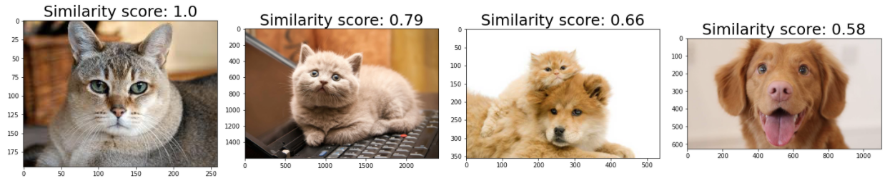
Here are two output examples.
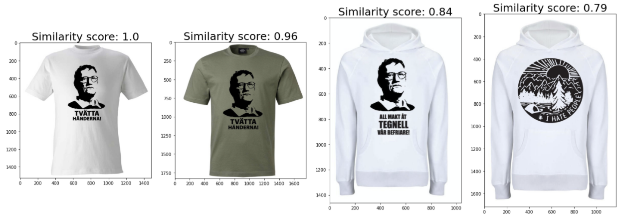
Explicitly controlled embedding. This method allows the feasibility to define the condition explicitly using the training data. For example, if the condition of the similarity is based on the color, we define red-red images as similar, and red-green images as dissimilar. Therefore you can supervise the model training to fulfill your condition. Below is an example using the triplet loss function to drive the model training.
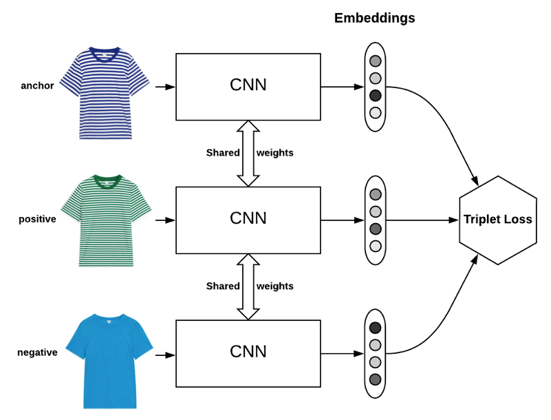
The Siamese neural network architecture is composed of 3 identical neural networks, which share the weights. By feeding the triplet of (anchor, positive, negative) samples, the triplet loss function is minimized in the training, where the triplet loss is defined as \(L(a, p, n) = \max \{d(a_i, p_i) - d(a_i, n_i) + {\rm margin}, 0\}\) and \(d(x_i, y_i) = \left\lVert {\bf x}_i - {\bf y}_i \right\rVert_p\)
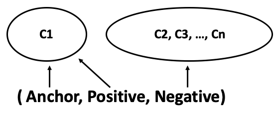
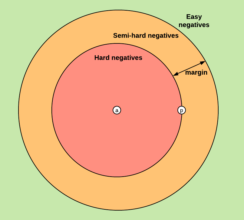
The strategy of triplet sampling is shown above, where we sample the anchor and positive from the same class, and the negative randomly from other classes. However we need to be aware of the pitfalls of hard, semi-hard, easy triplets as defined below. See more details in Olivier Moindrot’s blog.
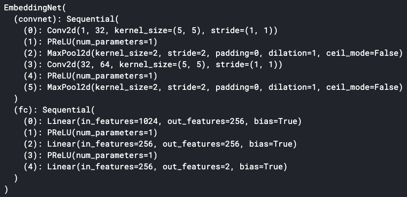
In this article, a shallow neural network is chosen to speed up the training process as well as to demonstrate the power of this triplet idea even though the neural network is pretty simple. To facilitate the visualization of the embedding, we use a 2-dimension embedding space. The embedding net is shown below:
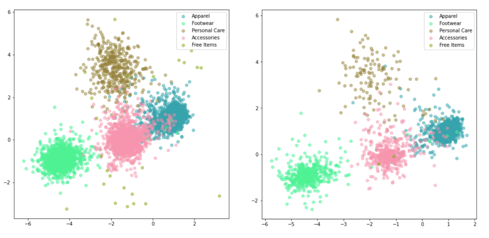
This output example sets the condition as “masterCategory”.
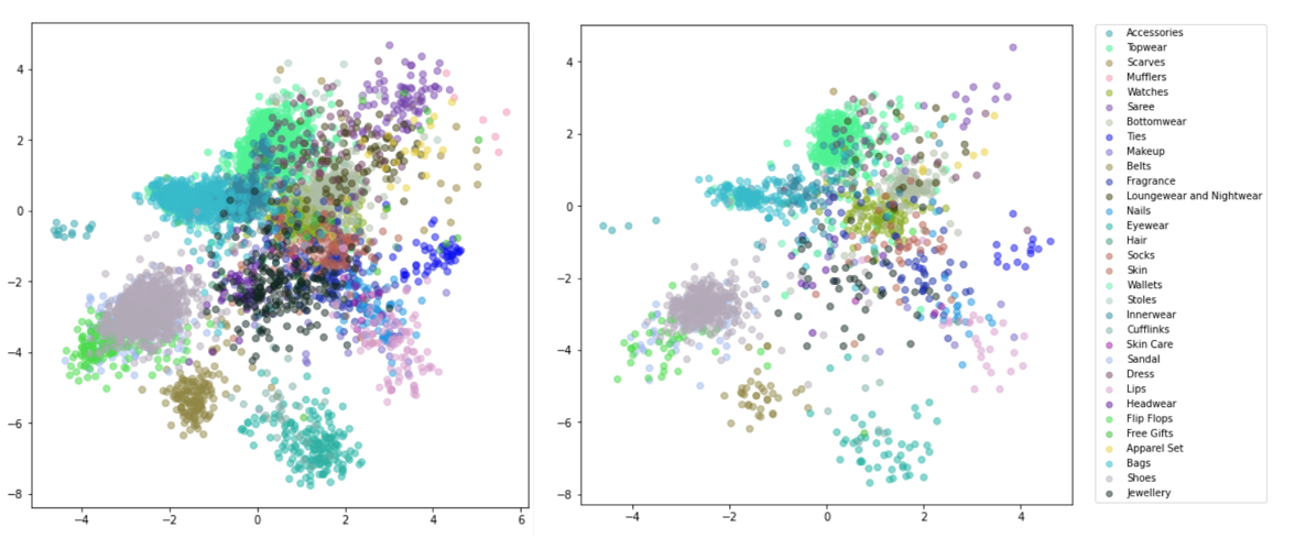
This output example sets the condition as “subCategory”.
How to measure the quality of the embeddings?
To measure the quality of the embedding, the test set can be constructed as long as the condition is well-defined. For example, if the color is used as the condition, test sets can be (red, red, similar), (red, green, dissimilar) and so on.
Summary
In this article, I illustrated that why a definition of the conditional visual similarity is required to have a quantitative discussion and measure of the similarity. Additionally both un-supervised and supervised methods are applied to generate the embedding space. Finally even though the quality of the embedding strongly depends on the image quality and training details, it can still be measured in a quantitative way if the condition is well-defined.