An introduction to time series analysis
Introduction
Time series analysis (TSA) provides us with an elegant framework to handle any dataset that contains the temporal ingredient. It serves a wide range of purposes, such as forecasting, time series classification, signal estimation, time series segmentation, exploratory analysis and more. All these techniques can be applied to various of data science and engineer problems. Among them, forecasting has been one of the most critical applications in many industry, such as demand forecast. Therefore TSA is an essential toolset to master.
After quickly reading through some theoretical textbooks and practical hands-on tutorials, I decided to write down my understanding here, with the focus on the times series fundamentals and forecasting.
Time series analysis
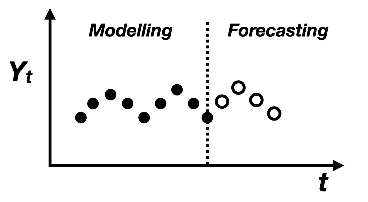
A time series is basically a series of data points indexed in time order, as shown in the figure above. The data points are correlated to some degree, otherwise they are just random noise.
This blog will limit the discussion around univariate and discrete time series.
Broadly speaking, time series analysis can be broken down into:
-
Time series modelling, which comprises methods for analyzing time series data in order to extract meaningful statistics and other characteristics of the data. -
Time series forecasting, which is the use of a model to predict future values based on previously observed values.
Time series modelling
Stochastic process
The sequence of random variable \(\{Y_t: t=0,1,2,...\}\) or more simply denoted by
\(\{Y_t\}\) is called a stochastic process, which can be described as “a statistical
phenomenon that evolves through time according to a set of probabilistic laws”.
A complete probabilistic time series model for \(\{Y_t\}\) would specify the joint cumulative distribution function (CDF): \(P(Y_1 \leq y_1, Y_2 \leq y_2,...,Y_n \leq y_n)\).
However this specification is not generally needed in practice. Much of the important information in most time series processes is captured in the first and second moments: \(E(Y_t)\) and \(E(Y_tY_{t-k})\).
Here are some important statistics for a stochastic process:
-
The mean function: \(\mu = E(Y_t)\)
-
The auto-covariance function: \(\gamma_{t,s} = cov(Y_t, Y_s) = E(Y_t Y_s) - E(Y_t)E(Y_s)\)
-
The auto-correlation function: \(\rho_{t,s} = corr(Y_t, Y_s) = \frac{cov(Y_t, Y_s)}{\sqrt(var(Y_t) var(Y_s))} = \frac{\gamma_{t,s}}{\sqrt(\gamma_{t,t} \gamma_{s,s})}\)
Famous stochastic processes
- A stochastic process \(\{e_t: t=0,1,2,...\}\) is called a white noise process if \(e_t\) is an independent and identically distributed (IID) random variable, with \(E(e_t) = \mu_e\) and \(var(e_t) = \sigma^2_e\).
Note that both are constant (free of \(t\)) and practically a white noise process can be simulated by \(e_t \sim iid~N(0, \sigma^2)\).
For a time series process \(\{Y_t\}\), it generally contains two types of variations:
- Systematic variations, such as trend, seasonality etc.
- Random variation (noise).
Therefore the white noise process can be used to
- Check if the time series is predictable or just noise.
- Diagnostic of the quality of the model fit (see the model fit discussion below).
-
Random walk process: \(Y_t = Y_{t-1} + e_t\)
-
Moving average process: \(Y_t = \frac{1}{3}(e_t + e_{t-1} + e_{t-2})\)
-
Autoregressive process: \(Y_t = \phi Y_{t-1} + e_t\)
Stationarity
Strictly stationary
The stochastic process \(\{Y_t\}\) is strictly stationary if the joint distribution of \(Y_{t1}, Y_{t2},...,Y_{tn}\) is the same as \(Y_{t1-k}, Y_{t2-k},...,Y_{tn-k}\) for all time points \(t_1, t_2,...,t_n\) and for all time lags \(k\).
It can be shown that this strictly stationary process has the following two properties:
- The mean function \(\mu_t = E(Y_t)\) is constant throughout time (free of \(t\)).
- The covariance between any two observations depends only on the time lag between them (\(\gamma_{t, t-k}\) depends only on \(k\), not on \(t\)).
Weakly stationary(second-order stationary)
Because strict stationarity is a condition that is much too restrictive for most applications. Moreover, it is difficult to assess the validity of this assumption in practice. A milder version is used instead: The stochastic process \(\{Y_t: t=0, 1, 2,..., n\}\) is said to be weakly stationary if it satisfied the above properties of the first two moments.
In weakly stationary case, nothing is assumed about the collection of joint distributions of the process.
-
Check for stationarity- Look at time series plots[quick and dirty]. Plot your time series and check if there is any obvious trends or seasonality.
- Summary statistics[quick and dirty]. Randomly split your data and check the obvious difference in statistics.
- Statistical test (Best). Such as Augmented Dickey-Fuller (ADF) test. More details Definition and Library.
-
Transform non-stationary to stationary. In order to apply most statistical methods, we need to transfer a non-stationary process into a stationary one. Here are some useful techniques:-
Differencing: By (repeatedly) doing differencing: \(Y'_{t} = Y_{t} - Y_{t-1}\) and then check the stationarity by ADF test.
-
De-trend and de-seasonality: Remove the trend or the seasonality by either differencing (above) or model fit. In the model fit approach, try to fit the time series with a linear or non-linear model, then subtract the model fit from the time series.
-
Decompose the time series: Decomposition provides us with an abstract model to interpret and analyze the time series. A times series is composed of (Level, Trend, Seasonality, Residual). They are modelled either additively: \(Y_t = L_t + T_t + S_t + R_t\) or multiplicatively: \(Y_t = L_t \times T_t \times S_t \times R_t\), which is equivalent to \(log Y_t = log L_t + log T_t + log S_t + log R_t\).
-
Time series forecasting
Time series forecasting can be done in two ways: classical statistical model like ARIMA or supervised machine learning models (see more discussion and A code example in Kats).
Classical statistical methods
ARIMA is a textbook-like classical statistical method. The forecasting process involves the following three steps.
-
Model selection: select model specification like \((p,d,q)\) in ARIMA
- Use ACF and PACF to get an idea of the values for \((p,d,q)\).
- Hyper-parameter tuning to select the best values of \((p,d,q)\).
-
Model estimation: fit the coefficients in the model
-
Model diagnostics
- Residual analysis: residuals are random quantities which describe the part of the variation in {Y_t} that is not explained by the fitted model. We need to check:
- Normality: Visually histogram + Q-Q plot and Shapiro-Wilk test
- Independence: Visually plot the residuals to check any pattern and runs test
- Use ACF to check IID and normality: standardized residuals should be a white noise process.
- Overfitting
- Residual analysis: residuals are random quantities which describe the part of the variation in {Y_t} that is not explained by the fitted model. We need to check:
Supervised machine learning problem
Summary
I discussed the definition of time series and a few key properties of a time series with the focus on stationary. Moreover the general forecasting steps are sorted out with more reference.